Lesson 16 – The Building Residual Techniques of Income Capitalization (The Income Approach to Value)

We will discuss the building (improvement) residual technique in this Lesson, and the land residual technique in the next lesson. The Building Residual Technique is, “A capitalization technique used when land value is known and residual income to the building or improvement is capitalized to obtain the building or improvement value.”^* The building residual technique is used when the land value is known; the land residual technique is used when income to an improvement can be obtained. Both techniques are basically the same – starting with the total income imputable to the property, the income imputable to one of the components (land or improvements) is deducted, which leaves the income residual to the other component, which is then capitalized into value, using the appropriate valuation method and rate.

Property Tax Rule 8, previously covered in Lesson 5, “Definition of the Income Approach and Property Tax Rule 8”, states, regarding the income approach to value:

…. It is the preferred approach for the appraisal of improved real properties and personal properties when reliable sales data are not available and the cost approaches are unreliable because ….

In subsection (b) this topic is expanded:

(b) Using the income approach, an appraiser values an income property by computing the present worth of a future income stream. …. In practical application, the stream is usually either

…

(2) divided horizontally by projecting a perpetual income for land and an income for the economic life of the improvements, …

…

It is the horizontally divided income streams that we will primarily discuss in this Lesson and the next Lesson; in Lesson 18 we will learn about the income streams described in subsection (b)(1).

Residual techniques allow for capitalization of an income stream allocated to an investment component of unknown value once all investment components of known value have been satisfied. An appropriate capitalization rate is applied to the value of the known components(s) to derive the annual income needed to support the investment in that component. The annual income of the known component(s) is deducted from the net income before recapture and taxes to derive the residual income available to the unknown component. The residual income is capitalized using an appropriate capitalization rate to derive the present value of the unknown component. The final step is to add the value(s) of the known components(s) and the value of the residual component to derive a value indication for the total property.

In Lesson 15 we learned that the appropriate capitalization rate for land – which is theoretically assumed to exhibit a constant perpetual income stream, is a combination of a yield rate (Y_o) and an effective tax rate (ETR). As was mentioned in that Lesson, the appropriate capitalization rate for improvements must make an allowance for recapture (return OF the investment), as well as for yield (return ON the investment) and property taxes.

How an allowance for recapture is determined depends on the shape of the income stream to the improvement. If the income stream is forecast to be straight-line declining terminal, then the Capital Recovery Rate [CRR] – the rate for the recapture allowance – is the reciprocal of the Remaining Economic Life [REL] – that is, it is calculated by dividing the number one (1) by the REL. However, if the income stream is forecast to be level terminal, then the Capital Recovery Rate [CRR] – the recapture allowance – is at the sinking fund rate, based on Y_o, for the REL of the wasting asset – that is, the improvement’s REL.

Let's rephrase these previous paragraphs. The residual techniques we are discussing will be used for the valuation of improved properties – either actually improved, or with proposed improvements. Using a residual technique, (1) the appraiser must know what the property will earn, either as improved, or as it might be improved. (2) The appraiser needs to know the information necessary to develop the capitalization rates – the yield rate, the rate of capital recapture, and the effective tax rate. And (3) the appraiser must know the value of one of the components of the improved, or hypothetically improved, property – either a building value or a land value.

1. First determine the income the property will earn under the highest and best use.
2. Using “IRV”, determine the income imputable to the known value component:
   1. In the Building Residual Technique, you must know the land value, and then the land income is the land value times the land capitalization rate; I_L = R_L × LV, where the R_L = (Y_O + ETR).
   2. In the Land Residual Technique, you must know the building value, and then the building income is the building value times the building capitalization rate; I_B = R_B × BV, where the R_B = (Y_O + {1÷REL} + ETR) or RB = (Y_O + SFF_{YO,Ann,REL} + ETR).
3. Subtracting the income attributable to the known value component from the total property income leaves you with the income residual to the unknown value component.
4. Use "IRV" to capitalize the income residual to the unknown value component into value.
   • If you knew the land value, then your residual income is the income to the building; BV = I_B ÷ R_B, where the R_B = (Y_O + {1÷REL} + ETR) or the R_B = (Y_O + SFF_{YO,Ann,REL} + ETR).
   • If you knew the building value, then your residual income is the income to the land; LV = I_L ÷ R_L, where the R_L = (Y_O + ETR).
5. Adding the known component value to the value just derived will result in the total value.

* From the online IAAO Gloassary

Lesson 6, Characteristics of the Income Stream, discussed the shapes of five different income streams: (1) Constant Perpetual; (2) Level (or Constant) Terminal; (3) Straight-Line Declining Terminal; (4) Variable Income; and (5) Single Income Payment (Reversion). In this lesson we will apply appraisal methods to the first three of these primary income patterns. In subsequent lessons we will continue using these income streams, and also examine the last pattern, the Single Reversion Payment; in Lesson 19 we will conclude this area of discussion when we apply the Level Terminal annuity and the Reversion payment in the appraisal of leased personal property.

Lesson 8, Capitalization, discussed “IRV”, Income = Rate × Value, and also discussed the use of Factors and Multipliers, comparing them to Rates. We said that, from a purely theoretical point of view, a Rate could be thought of as the reciprocal of a Multiplier or Factor.

Lesson 10, Rates and Factors, further discussed the relationship between rates and factors.

Hereinafter, when we use the term, “Rate”, such as in “IRV”, I = R × V, “Income equals Rate times Value”, we may be using it as a multiplier, quotient, divisor (or denominator), or as the result of a calculation — a quotient or product.

• In I = R × V, a multiplication calculation, R and V are the multipliers, and I is the product.
• In R = I ÷ V, and R = Ant I ÷ SP, division calculations, R is the quotient, I is the dividend (or numerator), and V (or SP) is the divisor.
• In V = I ÷ R, another division calculation, V is the quotient, I is still the dividend, and R is now the divisor.

Moreover, when we use the term, “factor”, we will usually be referring to a number taken from a compound interest table. Sometimes a factor may be the addend, sum, minuend, subtrahend, or difference in an equation.

• In “SFF + i = PR”, the Sinking Fund Factor [SFF] and the interest rate [i] are the addends and the Periodic Repayment factor [PR] is the sum, the result of the calculation.
• In "PR − i = SFF”, PR is the minuend, i the subtrahend, and SFF is the difference, the result.

Both residual techniques – building and land – are basically the same: starting with the total income imputable to the property, the income imputable to one of the components (land or improvements) is deducted, which leaves the income residual to the other component, which is then capitalized into value.

The building residual technique is used when the land value is known but the improvement value is unknown. After processing the market income stream of the subject property to the Net Income Before deducting for recapture and property Taxes level [NIBT], the income imputed to the land is deducted. The residual income is attributable to the building and may be converted to an estimate of improvement value by capitalizing it using a building capitalization rate.

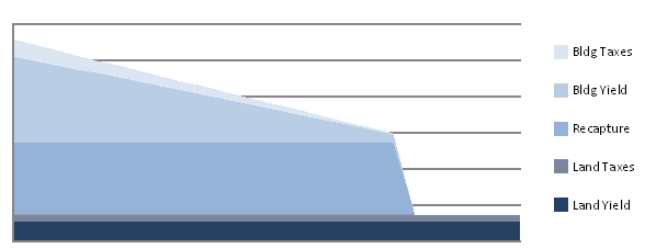
Building Residual Technique – Straight-Line Declining Terminal Income Stream

When the income stream is a series of annual incomes that decline in equal amounts over a period until the income of a wasting asset terminates, it is straight-line declining shaped. This premise assumes the net income declines by an equal amount each period, and as a result, the value declines an equal amount each period. The land income remains constant, and continues on into perpetuity. This is illustrated in the chart below – (1) the property taxes attributable to the improvements are a function of the improvement value, and therefore decline as the improvement value declines; (2) the return on investment (yield) attributable to the improvements is a function of the improvement value, and therefore decline as the improvement value declines; (3) the recapture of the investment in the improvement is an equal amount each year, until the entire improvement value has been recovered:

Information needed:

• Type of income stream, that is, straight-line declining terminal or level terminal
• Net Income Before deducting for recapture and property Taxes [NIBT], or the requisite information to derive NIBT
• Land Value [LV]
• Yield rate [Y]
• Effective Tax Rate [ETR]
• Remaining Economic Life of the building or improvements [REL]

After processing the market income stream to the Net Income Before deducting for Recapture and property Taxes level [NIBT], the income imputed to the land is deducted (Land Income). Land Income is derived by multiplying the Land Value by the factor created by the sum of the Yo plus the ETR. The residual income is attributable to the improvements (Improvement or Building Income). Dividing the Improvement Income by the capitalization rate, which is comprised of the Yo plus the CRR [ CRR ≡ 1 ÷ REL ] plus the ETR, will give us the Improvement Value. CRR can be derived by dividing the number one by the REL. Adding the Land Value to the Improvement Value will give us the Total Property Value.

This can also be expressed in the following format:

where:

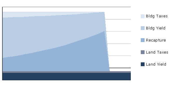
Building Residual Technique – Level Terminal Income Stream

When the income stream is a series of equal, annual incomes that terminate at some point in the future, the income stream is level terminal shaped. This income stream, attributable to the improvements, is a series of level, terminating payments; there is no reversionary value. This premise assumes that the value declines each period, but the net income remains constant. The land income remains constant, and continues on into perpetuity. This is illustrated in the following chart – (1) the property taxes attributable to the improvements are a function of the improvement value, and therefore decline as the improvement value declines; (1) the return on investment (yield) attributable to the improvements is a function of the improvement value, and therefore decline as the improvement value declines; (3) the amount of recapture of the investment in the improvement is based on the Sinking Fund Factor, and increases each year, until the entire improvement value has been recovered:

Information needed (they are the same as for the straight-line declining terminal premise):

• Type of income stream, that is, level terminal or straight-line declining terminal
• Net Income Before deducting for recapture and property taxes [NIBT], or the requisite information to derive NIBT
• Land Value [LV]
• Yield rate [Y]
• Effective Tax Rate [ETR]
• Remaining Economic Life of the buildings or improvements [REL]

After processing the market income stream to the Net Income Before deducting for Recapture and property Taxes level [NIBT], the income imputed to the land is deducted (Land Income). Land Income is derived by multiplying the Land Value by the factor created by the sum of the Yo plus the ETR. The residual income is attributable to the improvements (Improvement or Building Income). Dividing the Improvement Income by the capitalization rate, which is comprised of the Y_O plus the SFF plus the ETR, will give us the Improvement Value. The SFF is found at the Yield rate Y_O, Annual compounding, for the Remaining Economic Life of the improvements. Adding the Land Value to the Improvement Value will give us the Total Property Value.

This can also be expressed in the following formula:

Where:

The lesson you just read explained how to use residual techniques to value improved and vacant properties. The next lesson will address valuation the property reversion technique.