Lesson 14 – Review of Four Types of Income Streams and Methods of Capitalization (The Income Approach to Value)

A series of equal, annual incomes that flow into perpetuity. In theory, land is a non wasting asset and is capable of producing a constant perpetual income.

Here is how the Constant Perpetual Income Stream looks:

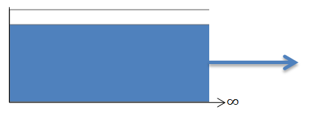
The blue area represents return ON investment. The income goes on into perpetuity.

"I R V" tells us that I = R × V, and V = I ÷ R. If the Income is Net Income [NI], then the capitalization Rate would be the Yield Rate [Y]; for the property tax appraiser, the Income would be the Net Income Before deducting for ad valorem property Taxes [NIBT], and the capitalization Rate would include the Effective Tax Rate [ETR] and the Yield Rate [Y].

Any series of equal, annual incomes that terminate at some point in the future.

Here is how the Level Terminal Income Stream looks:

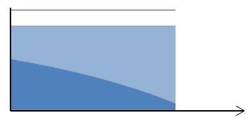
The blue area below represents return ON investment and the red area above represents recapture OF investment – capital recovery. The income terminates at the end of the Remaining Economic Life of the improvements, that is, when the improvements no longer have the ability to produce income.

"I R V" tells us that I = R × V, and V = I ÷ R. If the Income is Net Income Before deducting for Recapture [NIBR], then the capitalization Rate would include the Yield Rate [Y], to provide for return ON investment, and the Sinking Fund Factor [SFF], to provide for recapture OF investment; for the property tax appraiser, the Income would be the Net Income Before deducting for recapture and ad valorem property Taxes [NIBT], and the capitalization Rate would include the Yield Rate [Y], the Sinking Fund Factor [SFF], and the Effective Tax Rate [ETR].

Note that when we derived a level-terminal income stream yield rate in the previous lesson (Lesson 13, pages 6 – 8, including Example 13-2), we multiplied the Annuity Factor (PW1/P) times the NIBR – the Net Income Before deducting for Recapture (but after deducting the anticipated property taxes). In Example 14-2, above, there are property taxes; we capitalize NIBT into value using a "cap" rate that includes the ETR; PV = NIBT ÷ (Y + SFF_{Y,Ann,REL} + ETR)

When not appraising for ad valorem property tax purposes, the appraiser may deduct property taxes as an expense, and capitalizing NIBR (that is, NIBT less taxes – see Lesson 7, Net Income Before deducting Recapture, and Demonstrations 7-1 & 7-2). Use the same capitalization formula as in Example 14-2, except Income is NIBR, and ETR is zero. That is, V = I ÷ R = NIBT ÷ (Y + SFF_{Y,Ann,REL} + ETR) = NIBT ÷ (Y + SFF_{Y,Ann,REL} + 0) = NIBT ÷ (Y +SFF_{Y,Ann,REL} + ETR).

Continuing, say NIBT is $10,000, property taxes are $713.29, and therefore NIBR is $9,286.71. REL is still 10 years and Y is still 10%

The interrelationship between the factors in the compound interest and annuity tables were discussed in both Lessons 4 and 8. In particular, remember that the SFF plus the interest (yield) rate is the Periodic Repayment [PR] factor. Therefore, since ( i + SFF) = (Y + SFF) = PR, we could say:

Moreover, since the PR is the reciprocal of the annuity factor, PW1/P, we could multiply by the annuity factor rather than divide by the Periodic Repayment factor:

Does this work if we include the effective tax rate with the yield rate when we look up our factor? No, because it will affect the capital recovery portion that is built into the annuity and periodic repayment factors. The resulting answer will be close, but it will not be the same – here is Example 18-2 worked with the annuity factor and an 11¼%^† rate, that is 10% Y + 1¼ ETR:

Dividing by the 11¼%^†† Periodic Repayment factor (instead of multiplying by PW1/P), we calculate a similar result:

Summarizing the last two paragraphs, using a factor that includes both the yield and effective tax rates results in minor differences – about two percent in this instance, comparing the results ($58,280±) just above with the result in Example 14-2 ($57,063). The solution as shown in Example 14-2 is more accurate, and is preferred.

A series of annual net incomes that decline in equal amounts over time until the income terminates.

Here is how the Straight-Line Declining Terminal Income Stream looks:

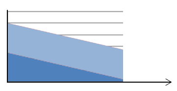
The blue area below represents return ON investment and the red area above represents recapture OF investment – capital recovery. The income goes on into perpetuity.

"I R V" tells us that I = R × V, R = I ÷ V, and V = I ÷ R. If the Income is Net Income Before deducting for Recapture [NIBR], then the capitalization Rate would include the Yield Rate [Y], to provide for return ON investment, and the Capital Recovery Rate [CRR], to provide for recapture OF investment;  for the property tax appraiser, the Income would be the Net Income Before deducting for recapture and ad valorem property Taxes [NIBT], and the capitalization Rate would include the Yield Rate [Y], the Capital Recovery Rate [CRR], and the Effective Tax Rate [ETR].

A lump sum payment the investor will receive at some point in time in the future.

Here is how a Single Reversion Payment looks:

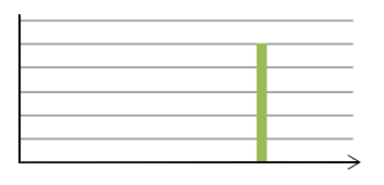
There is only a single payment, made once in the future.

Earlier in this lesson we talked about "IRV" and "VIM"; a third mnemonic is "VIF", "Value = Income × Factor". That is,
for “V I F”,
• V = I × F.

The Factor comes out of a compound interest and annuity tables, such as the BOE's AH 505, Capitalization Formulas and Tables. The "Reversion Factor" is the Present Worth of 1 [PW1], which indicates the present value of a single future income payment, and is used in estimating the value of a reversionary interest. "V I F" tells us that V = I × F. The Income is a single payment to be received in the future, and the Factor is found in the Present Worth of 1 column, at the yield rate, with annual compounding, for the number of years until the Income is received; for the property tax appraiser, the factor would be found at a rate which is the sum of the yield rate and the Effective Tax Rate.

The lesson you just read reviewed four basic income streams, and the related methods of capitalization. The next lesson will address land valuation.