This lesson serves as an introduction to the topic and discusses the following:
The objectives of this learning session are to:
In this learning session, instruction is provided through structured reading and illustrated examples. To assist in the attainment of the learning objectives, examples are incorporated within the lessons to illustrate the concept being discussed. Problems available at the end of lessons are to be worked by participants to ensure comprehension of concepts and calculations discussed in the lesson. A final examination is also available at the conclusion of this session, in order that certified property tax appraisers employed by a California County Assessors Office or the Board of Equalization may demonstrate their overall comprehension of the subject matter, attest to their participation in the learning session and receive training credit for completion of the session.
It´s intuitive to most people that a dollar today is preferable to a dollar to be received in the future. (Think about $1,000,000 today compared to $1,000,000 to be received 5 years from today. Which would you rather have?)
A dollar today can be invested to accumulate to more than a dollar in the future, which also makes a future dollar worth less than a dollar today. Hence, money has a time value. More generally, the time value of money is the relationship between the value of a payment at one point in time and its value at another point in time as determined by the mathematics of compound interest.
Because of the time value of money, payments made at different points in time cannot be directly compared. The compound interest functions—the mathematics of the time value of money – allow us to bring the payments to the same point in time for comparison purposes.
Time value of money calculations have wide application in finance, real estate, and personal financial decisions.
An understanding of them is essential in the field of valuation. There are several situations in real estate where dollars
at different points in time are compared:
The process by which payments (or cash flows) are moved forward in time is called compounding.
The process by which payments (or cash flows) are moved backward in time is called discounting.
All time value of money calculations involve either compounding or discounting — that is, moving amounts either forward or backward in time.
A series of cash flows can be graphically represented using a cash flow timeline. A timeline depicts the timing and amount of the cash flows.
For example, the following timeline depicts cash inflows of $100 to be received at the end of each of the next 5 years:
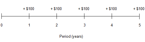
Cash flows in a timeline are often labeled positive or negative. By convention, positive cash flows correspond to cash inflows; negative cash flows correspond to cash outflows.
Whether a cash flow is an inflow or an outflow depends on perspective (i.e., as a borrower or lender). The borrower´s inflow is the lender´s outflow, and vice versa.
In using timelines, and in solving time value of money problems, one should adopt the perspective of either borrower or lender and stay with that perspective throughout the problem.
Consider a simple time value of money problem. In making a purchase you are given two payment alternatives:
As depicted on a cash flow timeline:
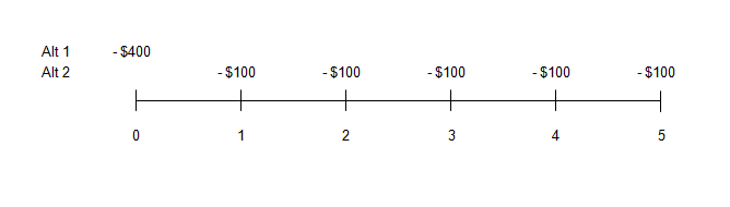
In deciding which alternative is better, we can´t simply add up the five payments of $100 and compare this sum ($500) with alternative 1 ($400 today). To do so would ignore the time value of money because the two alternatives involve payments at different times. Instead, we must determine the value today (at time 0) of the five future payments of $100 of alternative 2 and compare this to $400, which is the value today of alternative 1. As we shall see, determining the value today (the present value) of the five payments under alternative 2 involves calculating the present value of those payments at a given rate of interest.
Time value of money calculations allow us to solve problems such as the one above and many others.
When money is borrowed, the amount borrowed is called the principal. The consideration paid for the use of money is called interest.
Simple Interest
Simple interest refers to the situation in which interest is calculated on the original principal amount only.
With simple interest, the base on which interest is calculated does not change, and the amount of interest earned each period also does not change.
Compound Interest
Compound interest refers to the situation in which interest is calculated on the original principal and the accumulated interest.
With compound interest, interest is calculated on a base that increases each period, and the amount of interest earned also increases with each period.
Application of Simple Interest
Suppose someone invests $100 for 50 years and receives 5% per year in simple interest. To calculate simple interest, multiply the beginning balance by the rate 0.05 × $100 = $5. The growth in the investment is depicted in the table below:
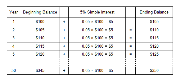
With simple interest, each year´s interest is based on the original principal amount only.
Application of Compound Interest
Assume the same investment of $100 for 50 years, but at compound interest:
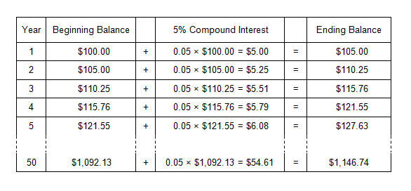
With compound interest, interest is earned on both the original principal and accumulated interest. Interest is earned on interest.
In the preceding example, with simple interest, the accumulated amount after 50 years is only $350. With compound interest, the accumulated amount is $1,147. As the term increases, the difference between the final amount with compound interest versus simple interest becomes more and more dramatic.
"Miracle of Compound Interest"
In a well-known transaction, Dutch colonists bought Manhattan Island in 1624 for the equivalent of $24.
From a lender´s (or investor´s) perspective, compound interest is a good thing; the lender earns interest on interest from the borrower.
Conversely, from a borrower´s perspective, compound interest is not so good.
The borrower, in effect, pays interest on interest throughout the term of the loan.
Compound Interest Functions
Six compound interest functions are used to solve time value of money problems. Not surprisingly, all of the functions are based on compound, not simple, interest. Each compound interest function is defined by a formula, which is the basis for calculating the compound interest factors for that function. Each formula requires a periodic interest rate and the number of periods
Most time value of money problems involve the use of only one compound interest function (or factor), but some require the use of two or more.
Understanding the compound interest functions, and how the factors derived from them are used to solve time value of money problems, is the heart of this subject matter. Each compound interest formula, and the factors derived from it, involves three variables:
In essence, using a compound interest factor does one of two things:
Published tables of compound interest factors are used to solve time value of money problems. It´s easier to refer to a table of
factors than to calculate the desired factor from one of the formulas each time you need it.
Time value of money problems can also be solved using a financial calculator or spreadsheet software. Essentially, the software calculates the necessary factor and processes the calculation.
We approach the subject by first showing how compound interest factors are derived from each of the formulas, then showing how the factors are used to solve various time value of money problems.
This approach provides a fundamental understanding of the material and a good basis for later using financial calculators and spreadsheet applications to solve time value of money problems.
The six compound interest functions are listed below; the following table briefly describes each function and gives an example of how it might be used.
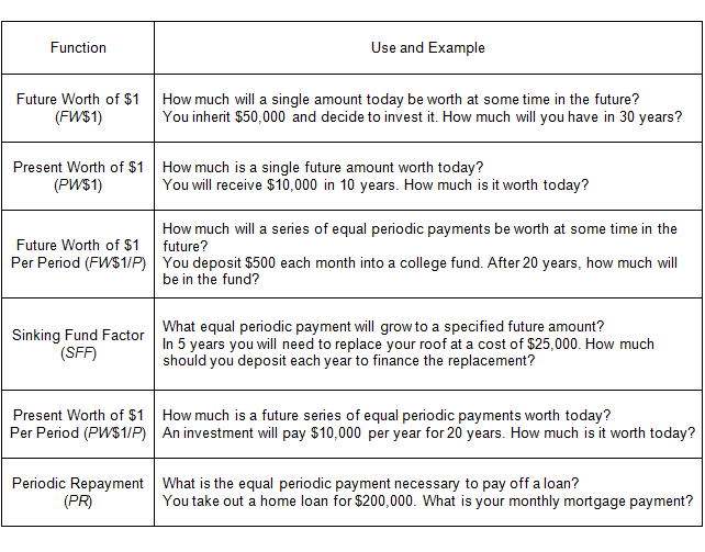
Review the above table as an introduction to the compound interest functions. Note that the first two compound interest functions (FW$1 and PW$1) deal with a single amount, or payment, while the remaining four deal with a series of payments (an annuity). Although all of the compound interest functions have appraisal applications, two are of particular importance because of their central role in the income approach – the present worth of $1 (PW$1) and the present worth of $1 per period (PW$1/P).
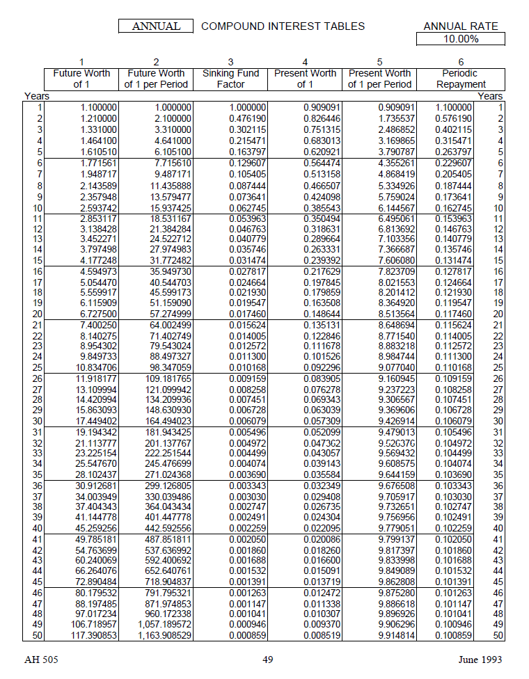
Assessors´ Handbook Section 505 (AH 505), Capitalization Formulas and Tables, contains a set of compound interest factors for use by property tax appraisers.
Briefly look through AH 505 (Use browser's back button to return to lessons).
To use the AH 505 tables, follow these steps:
(For solving the examples, we have recreated portions of the AH505 tables. We also provide a link to the actual pages in AH 505. If you go to an actual page, use the zoom feature for the best view.)
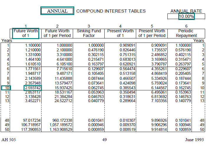
Example 1:
Find the FW$1 factor at 10% for 10 years, given annual compounding.
Solution:
In AH 505:
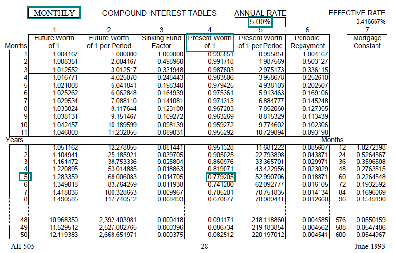
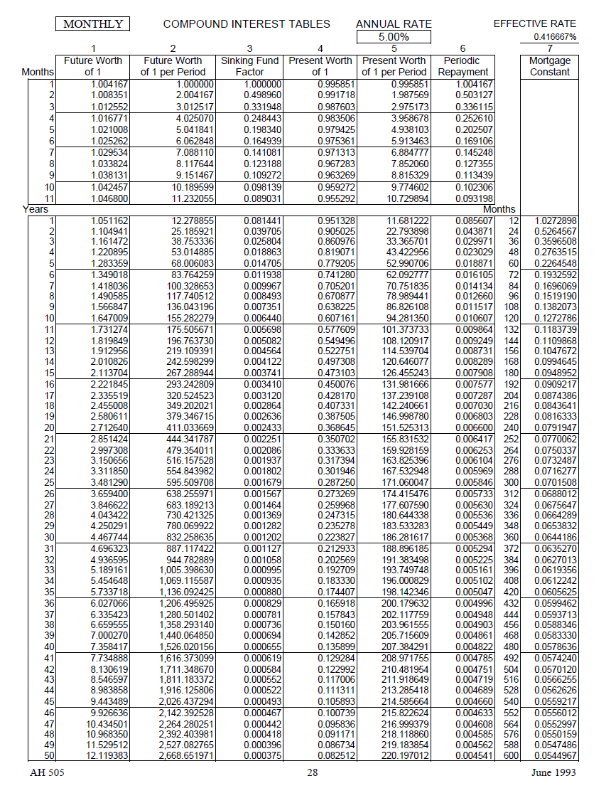
Example 2:
Find the PW$1 factor at 5% for 5 years, given monthly compounding.
Solution:
In AH 505:
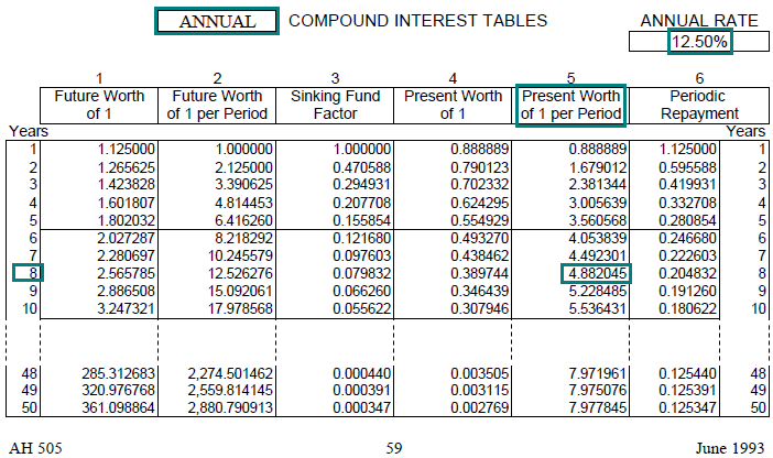
Example 3:
Find the PW$1/P factor at 12.5% for 8 years, given annual compounding.
Solution:
In AH 505:


